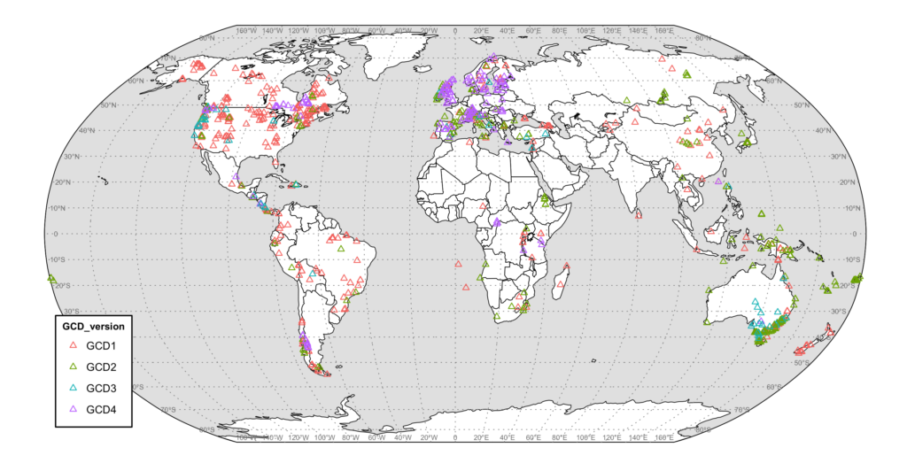

We are please to announce that the GCD and paleofire R packages have been updated to their 4.0.2 and 1.2.2 versions, respectively. GCD major update from 3.X.X to 4.X.X version number is associated to extensive changes in the way data is added into the package. GCD 4.X.X is now mirroring the online GCD SQL database on a monthly basis or whenever a significant number of new charcoal sites are added to the database.
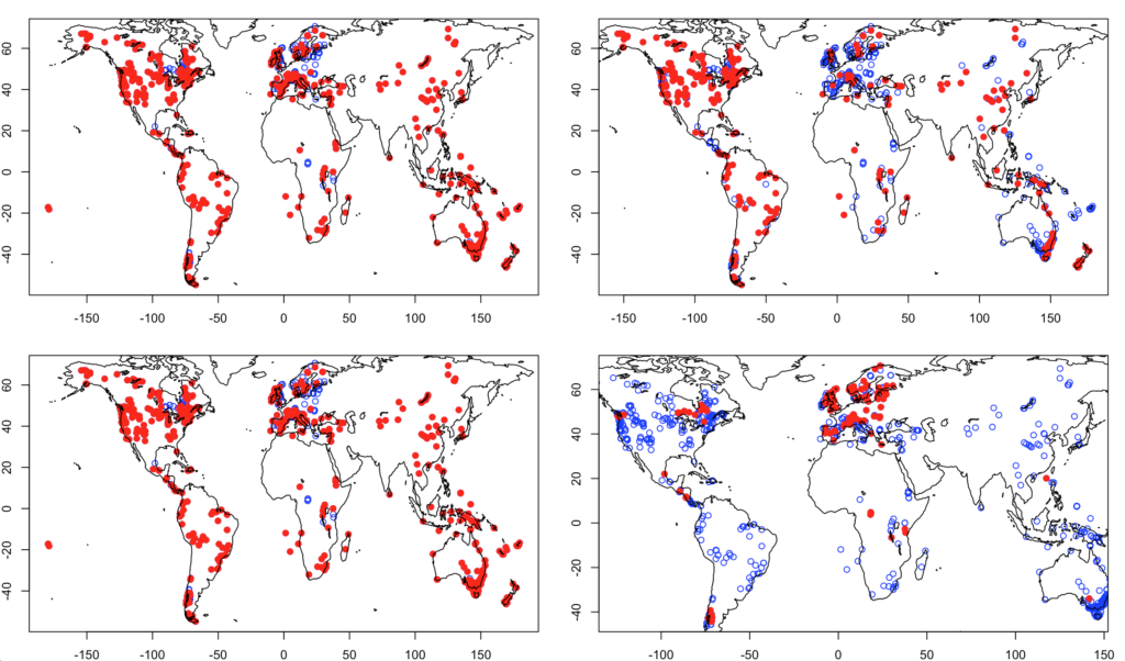
Three new fields in the paleofiresites table (see ?paleofiresites for details) enable to perform analyses with specific database versions or enable to select sites according to the date at which they have been added into the database. See the quick example below for explanations:
[code language=”R”]
par(mfrow=c(2,2))
plot( pfSiteSel(num_version < 400 ) ) # All sites in GCD version before 4.0.0
plot( pfSiteSel(gcd_version == "GCD1" ) ) # All sites in GCDv1
plot( pfSiteSel(update_date < "2016-01-01" ) ) # Sites included before 2016-01-01
plot( pfSiteSel(update_date &gt; "2018-01-01" ) ) # Sites included since 2018-01-01</code>
[/code]
The map above that is used to display all GCD charcoal sites has been produced by adapting the code available at https://seethedatablog.wordpress.com/2016/12/23/r-simple-world-map-robinson-ggplot/ please follow that link for additional references and explanations. The modified code is copied below:
[code language=”R”]</pre>
# ======================================================================================
# Create a simple world map in Robinson projection with labeled graticules using ggplot
# ======================================================================================
# Set a working directory with setwd() or work with an RStudio project
# __________ Set libraries
library(rgdal) # for spTransform() & project()
library(ggplot2) # for ggplot()
library(paleofire) #
setwd("/Users/OlivierB/Documents/R_in_progress/MAP_GCD/")
# __________ Load ready to use data from GitHub
load(url("https://github.com/valentinitnelav/RandomScripts/blob/master/NaturalEarth.RData?raw=true"))
# This will load 6 objects:
# xbl.X & lbl.Y are two data.frames that contain labels for graticule lines
# They can be created with the code at this link:
# https://gist.github.com/valentinitnelav/8992f09b4c7e206d39d00e813d2bddb1
# NE_box is a SpatialPolygonsDataFrame object and represents a bounding box for Earth
# NE_countries is a SpatialPolygonsDataFrame object representing countries
# NE_graticules is a SpatialLinesDataFrame object that represents 10 dg latitude lines and 20 dg longitude lines
# (for creating graticules check also the graticule package or gridlines fun. from sp package)
# (or check this gist: https://gist.github.com/valentinitnelav/a7871128d58097e9d227f7a04e00134f)
# NE_places – SpatialPointsDataFrame with city and town points
# NOTE: data downloaded from http://www.naturalearthdata.com/
# here is a sample script how to download, unzip and read such shapefiles:
# https://gist.github.com/valentinitnelav/a415f3fbfd90f72ea06b5411fb16df16
# __________ Project from long-lat (unprojected data) to Robinson projection
# spTransform() is used for shapefiles and project() in the case of data frames
# for more PROJ.4 strings check the followings
# http://proj4.org/projections/index.html
# https://epsg.io/
PROJ <- "+proj=robin +lon_0=0 +x_0=0 +y_0=0 +ellps=WGS84 +datum=WGS84 +units=m +no_defs"
# or use the short form "+proj=robin"
NE_countries_rob <- spTransform(NE_countries, CRSobj = PROJ)
NE_graticules_rob <- spTransform(NE_graticules, CRSobj = PROJ)
NE_box_rob <- spTransform(NE_box, CRSobj = PROJ)
# Add lakes http://www.naturalearthdata.com/http//www.naturalearthdata.com/download/10m/physical/ne_10m_lakes.zip
download.file("http://www.naturalearthdata.com/http//www.naturalearthdata.com/download/10m/physical/ne_10m_lakes.zip", destfile="ne_10m_lakes.zip")
unzip("ne_10m_lakes.zip")
NE_lakes <- readOGR(‘ne_10m_lakes.shp’,
‘ne_10m_lakes’)
NE_lakes <- spTransform(NE_lakes, CRSobj = PROJ)
NE_lakes <- NE_lakes[NE_lakes@data$scalerank==0,]
# project long-lat coordinates for graticule label data frames
# (two extra columns with projected XY are created)
prj.coord <- project(cbind(lbl.Y$lon, lbl.Y$lat), proj=PROJ)
lbl.Y.prj <- cbind(prj.coord, lbl.Y)
names(lbl.Y.prj)[1:2] <- c("X.prj","Y.prj")
prj.coord <- project(cbind(lbl.X$lon, lbl.X$lat), proj=PROJ)
lbl.X.prj <- cbind(prj.coord, lbl.X)
names(lbl.X.prj)[1:2] <- c("X.prj","Y.prj")
data("paleofiresites")
# Project GCD sites
gcd_rob=project(cbind(paleofiresites$long,paleofiresites$lat),PROJ)
gcd=data.frame(long=gcd_rob[,1],lat=gcd_rob[,2],GCD_version=paleofiresites$gcd_version)
# __________ Plot layers
ggplot() +
# add Natural Earth countries projected to Robinson, give black border and fill with gray
geom_polygon(data=NE_box_rob, aes(x=long, y=lat), colour="black", fill="grey90", size = 0.25) +
geom_polygon(data=NE_countries_rob, aes(long,lat, group=group), colour="black", fill="white", size = 0.25) +
geom_polygon(data=NE_lakes, aes(long,lat, group=group), colour="black", fill="white", size = 0.25) +
# Note: "Regions defined for each Polygons" warning has to do with fortify transformation. Might get deprecated in future!
# alternatively, use use map_data(NE_countries) to transform to data frame and then use project() to change to desired projection.
# add Natural Earth box projected to Robinson
geom_polygon(data=NE_box_rob, aes(x=long, y=lat), colour="black", fill="transparent", size = 0.25) +
# add graticules projected to Robinson
geom_path(data=NE_graticules_rob, aes(long, lat, group=group), linetype="dotted", color="grey50", size = 0.25) +
# add graticule labels – latitude and longitude
geom_text(data = lbl.Y.prj, aes(x = X.prj, y = Y.prj, label = lbl), color="grey50", size=2) +
geom_text(data = lbl.X.prj, aes(x = X.prj, y = Y.prj, label = lbl), color="grey50", size=2) +
# the default, ratio = 1 in coord_fixed ensures that one unit on the x-axis is the same length as one unit on the y-axis
geom_point(data=gcd, aes(long,lat, col= GCD_version),pch=2)+
coord_fixed(ratio = 1) +
# remove the background and default gridlines
theme_void()+
theme(legend.title = element_text(colour="black", size=8, face="bold"), # adjust legend title
legend.position = c(0.1, 0.2), # relative position of legend
plot.margin = unit(c(t=0, r=0, b=0, l=0), unit="cm"),
legend.background = element_rect(fill="white",
size=0.5, linetype="solid",
colour ="black")) # adjust margins
# save to pdf and png file
ggsave("map_draft_1.pdf", width=28, height=13.5, units="cm")
ggsave("map_1.png", width=26, height=13.5, units="cm", dpi=300)
# REFERENCES:
# This link was useful for graticule idea
# http://stackoverflow.com/questions/38532070/how-to-add-lines-of-longitude-and-latitude-on-a-map-using-ggplot2
# Working with shapefiles, projections and world maps in ggplot
# http://rpsychologist.com/working-with-shapefiles-projections-and-world-maps-in-ggplot
<pre>[/code]